Import Dynamic Data

Longitudinal (also called dynamic) networks are simply networks that evolve chronologically. If you imagine the network of your friends, the number of nodes, connections and attribute values grow and change as time passes. We call these dynamic attributes, because they have values associated with a particular moment.

Longitudinal Networks

There are two ways to model a longitudinal network, either a collection of networks where each network is a particular point in time (a day, a month, ...) or a slice network where each element has an interval of existence. This can also be described as Discrete vs. Continuous representations of time. Gephi uses the latter, also known as Intervals, because it's more flexible.

For example:

Imagine a network of three nodes for the years 2007, 2008 and 2009. The years these nodes are present can be represented either as distinct points in time or as time intervals (as pictured on the left and right sides of the arrow below, respectively).

The second node, 'n2', is present during all three years and is represented by brackets enclosing the first and last years [2007, 2009]. Gephi automatically includes any dates, such as 2008, within this range. The first node, 'n1', however, is closed with a parenthesis rather than a bracket. This means the node was present in 2008 but NOT in 2009.

Technically speaking, brackets are used for closed (also known as inclusive) intervals, while parentheses represent open intervals. In other words, dates enclosed within two brackets include both the startpoint and endpoint, whereas dates enclosed within two parentheses begins after the startpoint and ends before the endpoint. Half-closed intervals that incorporate both, like the [2007, 2009) example above, are also possible.

Check the Data Laboratory to see how intervals are created for each node or edge. When the network is longitudinal, a Time Interval column is present that shows when the interval is present in the graph. You can visualize this by clicking the checkbox next to 'Time intervals as graphics' in the Configuration tab of the Data Laboratory. After enabling the timeline, be sure to adjust the size of the window of the sliding filter of your timeline, otherwise you will receive an error stating that Gephi "cannot animate timeline without an animation interval."

Import from GEXF File

The GEXF format includes everything needed to represent longitudinal networks with intervals. You define a single network but add 'start' and 'end' attributes to set when a node/edge appears or vanish.

Basic example

Below is our earlier example with three nodes from 2007 to 2009, but we've added edges to complete the example graph.

<?xml version="1.0" encoding="UTF-8"?>
<gexf xmlns="http://www.gexf.net/1.1draft"
       xmlns:xsi="http://www.w3.org/2001/XMLSchema-instance"
       xsi:schemaLocation="http://www.gexf.net/1.1draft
                             http://www.gexf.net/1.1draft/gexf.xsd"
      version="1.1">
  <graph mode="dynamic" defaultedgetype="directed">
    <nodes>
      <node id="n1" label="Node 1" start="2007" endopen="2009" />
      <node id="n2" label="Node 2" start="2007" end="2009" />
      <node id="n3" label="Node 3" start="2008" end="2009" />
    </nodes>
    <edges>
      <edge source="n1" target="n2" />
      <edge source="n1" target="n3" start="2008"/>
      <edge source="n3" target="n2" start="2008" endopen="2009"/>
    </edges>
  </graph>
</gexf>

Notice the following important points:

• We set mode="dynamic" to the graph element, that is needed, as GEXF can represent static graphs as well
• Use start and end for closed intervals (ex: [2007, 2009]) and startopen and endopen for open (ex: (2008, 2009))
• Start and end dates for each element are optional. Leaving these empty will create an [-infinity, +infinity] interval. If only one bound is defined like for the second edge, it becomes [2009, +infinity].

The GEXF specifications, including dynamics, are available in the GEXF Primer.

Dynamic attributes

The example above described how to represent the network topology over time, where nodes and edges are added or remove. Now let's see how to represent values changing over time, for example 'Price'. Below is the same network with a price attribute. The attribute definition in the <attribute> element is the same as it would be for a static GEXF, but the way that values are written has changed.

<gexf xmlns="http://www.gexf.net/1.1draft"
      xmlns:xsi="http://www.w3.org/2001/XMLSchema-instance"
      xsi:schemaLocation="http://www.gexf.net/1.1draft
                          http://www.gexf.net/1.1draft/gexf.xsd"
                          version="1.1">
  <graph mode="dynamic" defaultedgetype="directed">
    <attributes class="node" mode="dynamic">
      <attribute id="price" title="Price" type="float"/>
    </attributes>
    <nodes>
      <node id="n1" label="Node 1" start="2007" endopen="2009" >
        <attvalues>
          <attvalue for="price" value="25.5" start="2007"/>
          <attvalue for="price" value="42.5" start="2008"/>
        </attvalues>
      </node>
      <node id="n2" label="Node 2" start="2007" end="2009" >
        <attvalues>
          <attvalue for="price" value="12" start="2008"/>
        </attvalues>
      </node>
      <node id="n3" label="Node 3" start="2008" end="2009" >
        <attvalues>
          <attvalue for="price" value="40.5" start="2008" end="2009" />
        </attvalues>
      </node>
    </nodes>
    <edges>
      <edge source="n1" target="n2" />
      <edge source="n1" target="n3" start="2008"/>
      <edge source="n3" target="n2" start="2008" endopen="2009"/>
    </edges>
  </graph>
</gexf>

Keep in mind the following

• To represent several values over time, the idea is to repeat the same attvalue for each period, with the same for but with different values and start/end
• It's not mandatory to set a value everywhere, in case of missing the default value is used
• For the node 'n2', the value '12' starts in 2008 and no end period is specified. That gives the interval [2008, +infinity] which means the value remains '12' in 2009 and after.

The GEXF specifications, including dynamics attributes are available in the GEXF Primer.

Dynamic weight

Normally an edge's weight is directly defined in the edge element with a particular value. Defining a dynamic weight attribute overrides this value and provides dynamic weight support.

The rule is to define an edge attribute with the weight keyword for identifier. Then, use multiple 'attvalue' like explained above to set different values over time.

<attributes class="edge" mode="dynamic">
   <attribute id="weight" title="Weight" type="float"/>
</attributes>

Transform existing column in Time Interval

Imagine a social network where each node represents a friend of yours and one of the attribute columns is the date you met. In order to transform this column into a dynamic interval take the following steps:

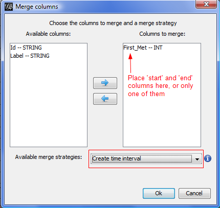
• Step 1: Click on Merge Columns manipulator in the Data Laboratory.

• Step 2: From the available columns on the left, add the column or columns (if you have both a start and end period) you want to use to create the time interval. Then select Create time interval from the available merge strategies.

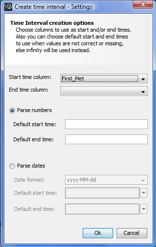
• Step 3: Select which column is the start and which is the end (or leave this blank if no end exists). If the column is numerical (integer, float, double), select Parse numbers. If the data are date strings, they can also be parsed and transformed into a time interval. Our 'First Met' column is just the day in the year, just a number.

Use Time Frame Import with several static files

NOTE: Outdated for Gephi 0.9.1, this documentation needs to be updated. Check https://github.com/gephi/gephi/issues/1546

This method can create a longitudinal network from a set of static "snaphsots" files. If you have a complete network at different point in time and want to see how both the network and its attributes changes over time this is the right method.

Note that this method implementation is still experimental and may not work in all cases. Be sure to verify the following points:

• Your node identifiers are exactly the same between the files. If not, at least the labels are (you can choose in the wizard).
• If GEXF, your network mode is set at static
• There is no previous graph in the workspace when you start importing Time Frame
• Attribute columns are the same in all files

Dataset

We can take for instance three GEXF files and say each of this file is for a particular year, the network in 2007, in 2008 and in 2009.

The static network in 2007, notice the price attribute:

<?xml version="1.0" encoding="UTF-8"?>
<gexf xmlns="http://www.gexf.net/1.1draft" version="1.1">
  <graph mode="static" defaultedgetype="directed">
    <attributes class="node" type="static">
      <attribute id="price" title="Price" type="int"/>
    </attributes>
    <nodes>
      <node id="1" label="Node 1">
        <attvalue for="price" value="12"/>
      </node>
      <node id="2" label="Node 2">
        <attvalue for="price" value="8"/>
      </node>
      <node id="3" label="Node 3">
        <attvalue for="price" value="5"/>
      </node>
    </nodes>
    <edges>
      <edge source="1" target="2" weight="1" />
      <edge source="1" target="3" weight="2" />
    </edges>
  </graph>
</gexf>

The static network in 2008, the node '3' disappeared and a node '4' appears. Prices and edge's weight have changed also.

<?xml version="1.0" encoding="UTF-8"?>
<gexf xmlns="http://www.gexf.net/1.1draft" version="1.1">
  <graph mode="static" defaultedgetype="directed">
    <attributes class="node" type="static">
      <attribute id="price" title="Price" type="int"/>
    </attributes>
    <nodes>
      <node id="1" label="Node 1">
        <attvalue for="price" value="15"/>
      </node>
      <node id="2" label="Node 2">
        <attvalue for="price" value="6"/>
      </node>
      <node id="4" label="Node 4">
        <attvalue for="price" value="8"/>
      </node>
    </nodes>
    <edges>
      <edge source="1" target="2" weight="4" />
      <edge source="1" target="4" weight="3" />
      <edge source="2" target="4" weight="1" />
    </edges>
  </graph>
</gexf>

The static network in 2009, the node '3' is back, the node '2' is gone and priced changed again.

<?xml version="1.0" encoding="UTF-8"?>
<gexf xmlns="http://www.gexf.net/1.1draft" version="1.1">
  <graph mode="static" defaultedgetype="directed">
    <attributes class="node" type="static">
      <attribute id="price" title="Price" type="int"/>
    </attributes>
    <nodes>
      <node id="1" label="Node 1">
        <attvalue for="price" value="10"/>
      </node>
      <node id="3" label="Node 3">
        <attvalue for="price" value="3"/>
      </node>
      <node id="4" label="Node 4">
        <attvalue for="price" value="12"/>
      </node>
    </nodes>
    <edges>
      <edge source="1" target="3" weight="5" />
    </edges>
  </graph>
</gexf>

Import in Gephi

Do the following steps on a clear project to import your dataset:

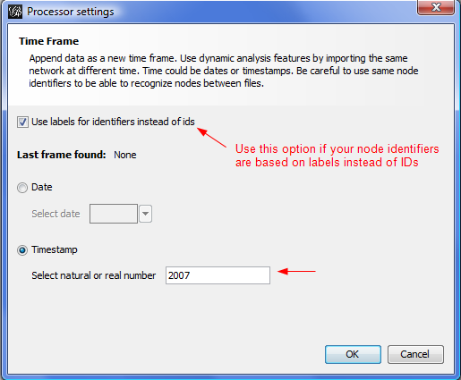
• Step 1: Import the first file and select Time Frame in the import report, click on OK. That will display a settings dialog.

• Step 2: Select either a Date or a real number as a time format. Real numbers is the default choice, here we put the year 2007. Click on OK, the file is imported.

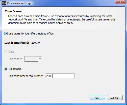
• Step 3: You can now do the same for all other files, in a chronological order. For the second file select 2008, then 2009 etc.

The result is a longitudinal network in Gephi where nodes and edges have time intervals according how they were present in the different files. Similarly all attributes are dynamic attributes. The 'Price' attribute in the dataset in a DYNAMIC_INTEGER column and each value is associated with its interval. Moreover the edge's weight itself is dynamic.